class: center, middle, inverse, title-slide .title[ # Useful stats functions and plots, text manipulation, regular expressions ] .author[ ### Mikhail Dozmorov ] .institute[ ### Virginia Commonwealth University ] .date[ ### 08-30-2023 ] --- ## Empirical Cumulative Distribution Function ```r set.seed(4) Fn <- ecdf(x <- rnorm(100)) # ?ecdf() curve(Fn) # Try plot(Fn) ``` 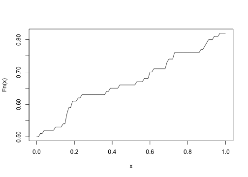<!-- --> --- ## Quantile-Quantile Plots - `qqnorm()`, `qqline()`, `qqplot()` - distribution comparison plots ```r data(trees) # load data to global environment attach(trees) qqnorm(Height) # A normal QQ plot ``` 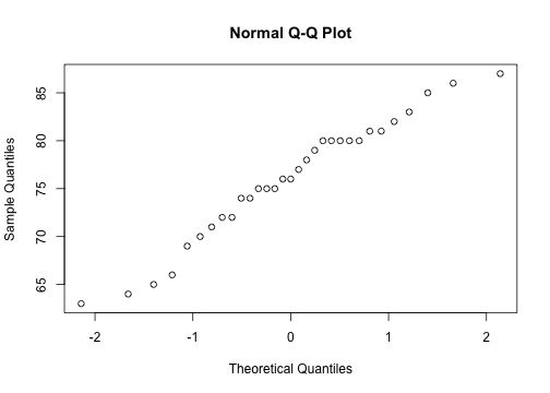<!-- --> --- ## Scatterplot Matrices - `pairs()` - pair-wise plot of multivariate data ```r data(trees) pairs(trees) ``` 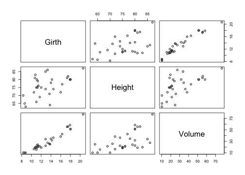<!-- --> --- ## Random samples and permutations ```r sample(1:10) ``` ``` ## [1] 7 5 10 2 1 4 8 3 9 6 ``` ```r sample(letters, 5) ``` ``` ## [1] "l" "q" "a" "v" "b" ``` ```r sample(1:10, replace = TRUE) ``` ``` ## [1] 1 6 10 5 2 2 8 10 10 3 ``` ```r set.seed(1) ``` --- ## Examples of density functions Prefix each R distribution name with "d" for the density or mass function, "p" for the CDF, "q" for the percentile function (also called the quantile), "r" for the generation of pseudorandom variables | Function | Distribution | |----------|--------------| | (d,p,q,r)norm | Normal | | (d,p,q,r)pois | Poisson | | (d,p,q,r)binom | Binomial | | (d,p,q,r)chisq | Chi-squared | | (d,p,q,r)t | Student's t | | (d,p,q,r)unif | Uniform | --- ```r x=rnorm(100) y=rnorm(100) plot(x, y) ``` 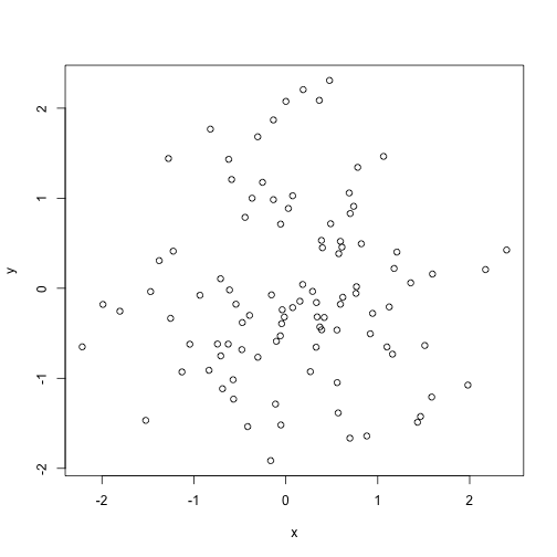<!-- --> ```r qnorm(.75,mean=10,sd=2) # 3rd quartile of N(mu = 10,sigma = 2) ``` ``` ## [1] 11.34898 ``` ```r qnorm(c(0.05, 0.10, 0.20, 0.95),mean=10,sd=2) ``` ``` ## [1] 6.710293 7.436897 8.316758 13.289707 ``` ```r qt(.95,df=20) # 95th percentile of t(20) ``` ``` ## [1] 1.724718 ``` --- ```r x<-rchisq(100,1) plot(x) ``` 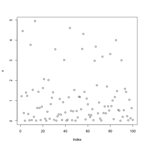<!-- --> ```r hist(x) ``` 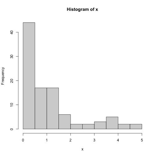<!-- --> ```r x<-dbinom(3:10,size=10,prob=.25) # P(X=3) for X ~ Bin(n=10, p=.25) barplot(x) ``` 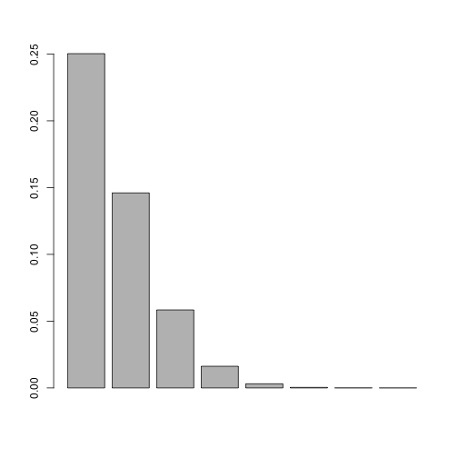<!-- --> ```r plot(x) ``` 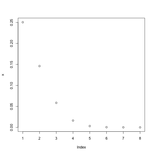<!-- --> ```r plot(0:10, dbinom(0:10, size=10, prob=.25), type = "h", lwd = 30) ``` 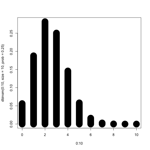<!-- --> ```r plot(3:10, x, type = "h", lwd = 30, main = "Binomial Probabilities w/ n = 10, p = .25", ylab = "p(x)") # which is gives the histogram-like vertical lines ``` 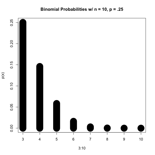<!-- --> ```r # lwd option (the default width is 1) controls line thickness ``` --- ```r dpois(0:2, lambda=4) # P(X=0), P(X=1), P(X=2) for X ~ Poisson ``` ``` ## [1] 0.01831564 0.07326256 0.14652511 ``` ```r x<- dpois(0:20, lambda=4) barplot(x) ``` 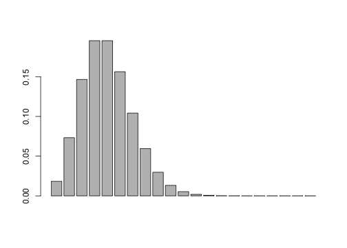<!-- --> ```r # plot(x) ``` --- ```r pbinom(3,size=10,prob=.25) # P(X <=3) in the above distribution ``` ``` ## [1] 0.7758751 ``` ```r x<- pbinom(3:10,size=10,prob=.25) plot(x) ``` 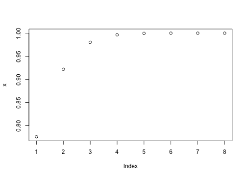<!-- --> --- ## More useful stats functions ```r lm(Sepal.Length~Sepal.Width, data=iris) # simple linear regression ``` ``` ## ## Call: ## lm(formula = Sepal.Length ~ Sepal.Width, data = iris) ## ## Coefficients: ## (Intercept) Sepal.Width ## 6.5262 -0.2234 ``` ```r glm(ifelse(Species=="setosa",1,0)~Sepal.Width, family="binomial",data=iris) # logistic regression ``` ``` ## ## Call: glm(formula = ifelse(Species == "setosa", 1, 0) ~ Sepal.Width, ## family = "binomial", data = iris) ## ## Coefficients: ## (Intercept) Sepal.Width ## -15.72 4.79 ## ## Degrees of Freedom: 149 Total (i.e. Null); 148 Residual ## Null Deviance: 191 ## Residual Deviance: 123.8 AIC: 127.8 ``` --- ## More useful stats functions ```r t.test(iris$Sepal.Length,iris$Petal.Length) ``` ``` ## ## Welch Two Sample t-test ## ## data: iris$Sepal.Length and iris$Petal.Length ## t = 13.098, df = 211.54, p-value < 2.2e-16 ## alternative hypothesis: true difference in means is not equal to 0 ## 95 percent confidence interval: ## 1.771500 2.399166 ## sample estimates: ## mean of x mean of y ## 5.843333 3.758000 ``` ```r aov(Sepal.Length~Species,data=iris) ``` ``` ## Call: ## aov(formula = Sepal.Length ~ Species, data = iris) ## ## Terms: ## Species Residuals ## Sum of Squares 63.21213 38.95620 ## Deg. of Freedom 2 147 ## ## Residual standard error: 0.5147894 ## Estimated effects may be unbalanced ``` --- ## More useful stats functions ```r chisq.test(iris$Petal.Length,iris$Species) ``` ``` ## Warning in chisq.test(iris$Petal.Length, iris$Species): Chi-squared ## approximation may be incorrect ``` ``` ## ## Pearson's Chi-squared test ## ## data: iris$Petal.Length and iris$Species ## X-squared = 271.8, df = 84, p-value < 2.2e-16 ``` ```r fisher.test(mtcars$gear, mtcars$carb) ``` ``` ## ## Fisher's Exact Test for Count Data ## ## data: mtcars$gear and mtcars$carb ## p-value = 0.2434 ## alternative hypothesis: two.sided ``` --- ## Regression models Regression models can be used to estimate how the expected value of a dependent variable changes as independent variables change. In R, regression formulas take this structure: ``` ## Generic code [response variable] ~ [indep. var. 1] + [indep. var. 2] + ... ``` Notice that a tilde, ~, is used to separate the independent and dependent variables and that a plus sign, +, is used to join independent variables. This format mimics the statistical notation: `\(Y_i \sim X_1 + X_2 + X_3\)` --- ## Conventions for linear models | Convention | Meaning | |:-----------:|:-------:| | I() | evaluate the formula inside I() before fitting (e.g., I(x1 + x2)) | | : | fit the interaction between x1 and x2 variables | | * | fit the main effects and interaction for both variables (e.g., x1*x2 equals x1 + x2 + x1:x2)| | . | include as independent variables all variables other than the response (e.g., y ~ .) | | 1 | intercept (e.g., y ~ 1 for an intercept-only model) | | - |do not include a variable in the data frame as an independent variables (e.g., y ~ . - x1); usually used in conjunction with . or 1 | --- ## Linear models To fit a linear model, you can use the function `lm()`. This function is part of the `stats` package, which comes installed with base R ```r mod <- lm(mpg ~ hp, data = mtcars) # Check class() and str() of the mod object ``` This previous call fits the model: `\(Y_{i} = \beta_{0} + \beta_{1}X_{1,i} + \epsilon_{i}\)` .small[ [INTRODUCTION TO LINEAR MIXED MODELS](https://ourcodingclub.github.io/tutorials/mixed-models/) ] --- ## Manipulating the `lm` object | Function | Description | |:---------:|:-----------:| | summary | Get a variety of information on the model, including coefficients and p-values for the coefficients | | coefficients | Pull out just the coefficients for a model | | fitted | Get the fitted values from the model (for the data used to fit the model) | | plot | Create plots to help assess model assumptions | residuals | Get the model residuals | ```r class(mod) ``` ``` ## [1] "lm" ``` --- ## plot(mod) 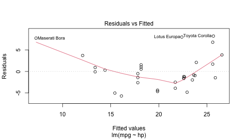<!-- -->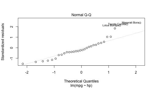<!-- -->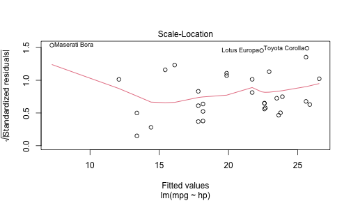<!-- -->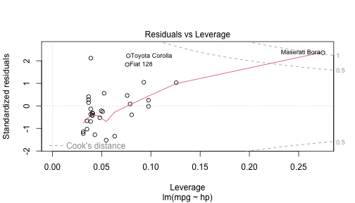<!-- --> --- ## Manipulating the `lm` object ```r mod_coef <- coefficients(mod) library(ggplot2) ggplot(mtcars, aes(x = hp, y = mpg)) + geom_point(size = 1) + xlab("Miles/(US) gallon") + ylab("Gross horsepower") + geom_abline(aes(intercept = mod_coef[1], slope = mod_coef[2]), col = "red") ``` 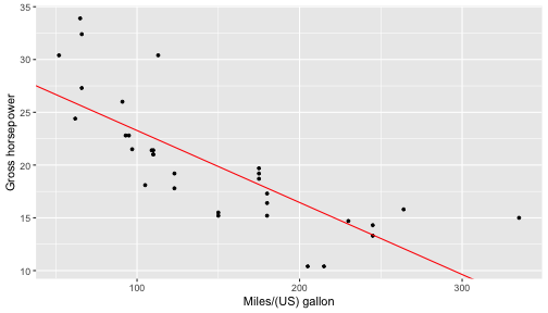<!-- --> --- ## Working with text - The `grep()` function takes as parameters the pattern and a character vector as the data to search through for the pattern. Parameters: - `ignore.case = FALSE` - by default it is case sensitive - `value = FALSE` - by default returns vector with index values of match; otherwise returns the values - `fixed = FALSE` - by default treats pattern as regular expression; otherwise will match exact - `invert = FALSE` - by default matches the pattern; otherwise returns what is not matched ```r strings <- c('abcd', 'dabc', 'abcabc') pattern <- '^abc' print (grep(pattern, strings)) ``` ``` ## [1] 1 3 ``` .small[`grepl()` - grep logical, returns a vector of the same length as a string, with TRUE/FALSE pattern matching] --- ## Regular expressions Some useful regular expression operators include: | Expression | Description | |:----------:|-------------------------------------------------------------------------------------------------------------------------------------------------| | [] | Matches a set. [abc] matches a, b, or c. [a-zA-Z] matches any letter. [0-9] matches any number. "^" negates a set, [^abc] matches d, e, f, etc. | | ^ | Starting position anchor. ^abc finds lines starting with abc | | "$" | Ending position anchor. xyz"$" finds lines ending with xyz. Remove quotes | | \\ | Escape symbol, to find special characters. \\\* will find \*. \\n matches new line character, \\t - tab character | | \* | Match the preceding element zero or more times. a\*b matches ab, aab, aaab, etc. | --- ## Extended regular expressions | Expression | Description | |:----------:|--------------------------------------------------------------------------------| | ? | Matches the preceding element zero or one time. a*b matches b, ab, but not aab | | + | Matches the preceding element one or more times. a+b matches ab, aab, etc. | | &#124; | OR operator. "abc&#124;def" matches abc or def | | . | Any character | --- ## Special characters | Expression | Description | |:----------:|--------------| | \\n | Newline | | \\r | Return | | \\t | Tab | [Curated Regular Expression Resources](https://paulvanderlaken.com/2020/04/07/curated-regular-expression-resources/) [Learn regex the easy way](https://github.com/ziishaned/learn-regex) [All about Regular Expressions](https://www.regular-expressions.info) [Preview your regex](https://regexr.com/) [Play Regex Golf](https://alf.nu/RegexGolf)